Background

Per- and polyfluoroalkyl substances (PFAS) are industrially-produced compounds that include chemicals such as perfluorooctanesulfonate (PFOS), perfluorooctanoate (PFOA), and newer replacements such as “GenX” and perfluorobutanesulfonic acid (PFBS). A central characteristic of this class of chemicals is the presence of a strong carbon-fluorine bond that resists chemical, thermal, and biological transformation. Some PFAS have been used extensively in consumer products and for industrial applications for several decades because of their unique physical and chemical properties: oil and water repellency, temperature resistance, and ability to reduce friction in a wide range of products. For example, some PFAS have been used in coatings for textiles, paper products and cookware, and in some firefighting foams. They have a range of applications in the aerospace, photographic imaging, semiconductor, automotive, construction, electronics, and aviation industries. Studies have shown that some PFAS can have potentially negative health effects, and, because of their persistence, they can bioaccumulate once released into the environment.

There are a wide variety of reported potential adverse health impacts associated with PFAS exposure, and active on-going debate about their toxicity and what constitutes a safe level. These chemicals can migrate into the air, dust, food, soil and are highly soluble in water.

One exposure route is through respiration (with some studies showing positive correlations between indoor dust levels of PFAS and human blood concentrations). A recent peer-reviewed paper¹ authored by EPA scientists identifies inhalation screening levels (ISLs) for four PFAS compounds (PFOA, PFOS, GenX, and PFBS) that are linked to drinking water health advisory levels, since a key exposure route is through ingestion of impacted drinking water. The water contamination can occur through direct runoff of PFAS compounds into the ground or water, as well as through atmospheric deposition from air emissions. With the availability of the ISLs noted above (1.5x10^-3, 7.9x10^-3, 3, and 300 ng/m³ for PFOA, PFOS, GenX, and PFBS, respectively), either air concentration levels or deposition levels can be used to assess impacts of PFAS air emissions. The availability of the air concentration route for PFAS impacts is the main update provided here for the air modeling approach, although we also provide guidance for the more complex deposition modeling approaches.

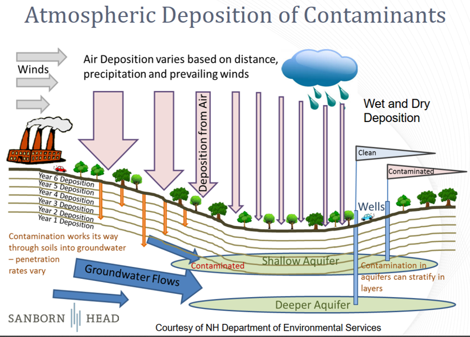
The figure below, from a recent EPA presentation, provides a depiction of PFAS fate and transport. This is an emerging topic and there is not yet an EPA-designated standard approach or consensus as to how best model PFAS air emissions. However, the discussion provided below takes advantage of existing practices and newly-developed modeling capabilities for PFAS compounds.

Air Modeling Overview

PFAS compounds that are emitted will persist in soil and water for several years after release, according to EPA authors that have recently completed air modeling of these compounds. While most PFAS compounds do not remain long in the atmosphere, air flow does allow for long-range transport (if there is not localized wet deposition), resulting in low ambient concentrations at any one location at large distances. A 2021 EPA study² indicates that peak airborne and deposition impacts occur close to the source, even though a large part of the emitted mass can travel tens or even hundreds of kilometers under favorable meteorological conditions. PFAS compounds have a very wide range of molecular weight, so the behavior may depend on the physical properties of the specific chemicals that are emitted. There is even the possibility that peak ground water concentrations can occur upstream of a PFAS source if the air transport would advect the PFAS emissions in that direction.

The focus of air modeling for airborne or deposition impacts is often localized due to peak short-range impacts, and can readily be accomplished using a short-range steady-state model such as AERMOD. However, for a complete impact assessment, or for complex winds situations, long-range photochemical grid (Eulerian) models such as CMAQ or CAMx, or Lagrangian puff models such as CALPUFF or SCICHEM could be used. The discussion below addresses how either type of modeling approach can be done.

Air Modeling Challenges

There are thousands of PFAS compounds with varying carbon-chain lengths, molecular weights and physical properties. For direct air concentration modeling, the fact that the compounds have different physical properties does not affect the modeling results because the straightforward modeling approach is to treat the emissions as a tracer with no deposition depletion. For states such as Michigan and New York that are instituting air toxics guidelines for PFAS airborne concentrations, AERMOD would be separately run with PFOA, PFOS, GenX, and PFBS compounds as a passive tracer. Use of the ISLs simplifies the modeling approach. For a more refined approach using deposition modeling, the approach is not as simple due to the difference in results between gas and particle deposition modeling approaches.

The EPA 2021 paper noted above, which focused upon a “CMAQ-PFAS” approach with a photochemical grid model, used an initial assumption that all PFAS compounds are emitted in the gaseous state. However, some PFAS in a gaseous state can transform to very small particles by solubility in small water droplets (or surface water bodies) or condensation into organic aerosols. In either case for gas-to-particle transition, the result is a very small particle, on the order of 1 micron in size. The CMAQ-PFAS approach provides the physicochemical properties of each model compound that are used to calculate the partitioning between the gas- and aerosol-phase components as well as the dissolution in cloud droplets and uptake to dry and aqueous land surface types.

The transport and fate of PFAS emissions is a function of the source, properties of the PFAS compound, and environmental conditions. The primary processes controlling the fate of PFAS in the environment are transport, partitioning, and transformation. In general, vapor pressures of PFAS are low and water solubilities are high, limiting transfer from water to air, though there are exceptions. However, PFAS can be transported through the atmosphere in both the gas and particle phases. The rate of deposition in dry periods is likely to be slow, but much more rapid for precipitation events, especially with the high water solubility of many PFAS compounds.

Long-range transport is responsible for the wide distribution of PFAS to all areas of the world; this has been confirmed by their occurrence in biota, surface snow, ice cores, seawater, and other environmental media in regions as remote as the Arctic and Antarctic. Distribution of PFAS to remote regions far removed from direct industrial input is believed to occur from long-range atmospheric transport as well as through ocean currents and being re-emitted into the air via sea spray, especially near coastlines.

One key issue relating to solubility of the emitted PFAS compounds is the potential conversion through hydrolysis within the production and emission process (or in the atmosphere after emission) of acyl fluorides with relatively low water solubility to carboxylic acids with high water solubility. This transformation will affect the deposition rate in the modeling. EPA’s 2021 study indicated that without the hydrolysis transformation being considered, the deposition rate was underestimated (mostly gas phase deposition), but it was overestimated with the assumption of instantaneous hydroloysis, resulting in the use of a higher Henry’s Law constant (which would result in more particle deposition).

Available Modeling Approaches for PFAS Deposition

AERMOD Modeling

The state of North Carolina has previously used AERMOD to model PFAS deposition by assuming the “Method 2” deposition approach with a mean particle size of 1.25 microns and a 0.944 fraction of particulate mass with a size less than 2.5 microns. This approach would likely lead to a conservatively high deposition rate because all of the emitted PFAS is assumed to be in the particulate form. With the availability of the inhalation screening levels, the use of AERMOD with gaseous emissions to determine air concentrations can now be used to assess the health consequences of airborne emissions of the key PFAS compounds of PFOA, PFOS, GenX, and PFBS.

CALPUFF Modeling

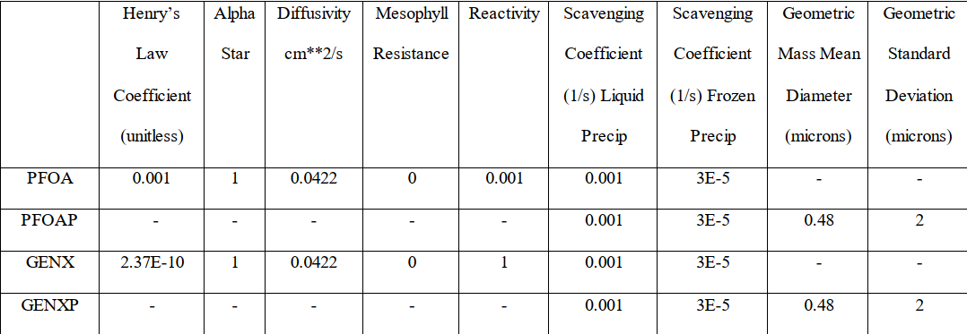
A 2019 Ohio State University Masters Thesis used CALPUFF as the model to simulate deposition of PFAS compounds. The emitted compounds were treated as both gases and particles in separate modeling runs, but could be subdivided in a single run. The chemical species parameters used in this study are listed in Table 1 (compound names ending in “P” are particles; otherwise gases). The use of CALPUFF has the advantage of using a 3-dimensional wind field input to optimize the transport modeling of the emissions as well as use of a gridded knowledge of surface characteristics that affect deposition rates. Again, with the availability of the inhalation screening levels, the use of CALPUFF with gaseous emissions to determine air concentrations can now be used to assess the health consequences of airborne emissions of the key PFAS compounds noted above.

Table 1: Chemical Properties Used in CALPUFF Deposition Modeling of Selected PFAS

Photochemical Grid Modeling

EPA has developed a new version of the photochemical grid model, CMAQ, with PFAS deposition capabilities (the model is called “CMAQ-PFAS”). The enhancements and grid model advantages include:

• An extensive physiochemical database of properties (molecular weight, density, saturation vapor concentration, heat of vaporization, and Henry’s Law constant) for numerous compounds.
• Use by CMAQ-PFAS of the physicochemical properties to predict gas-particle partitioning and influence rates of dry (removal of gases and particles to soil, vegetation, and other surfaces in the absence of precipitation) and wet (removal via rain, snow, fog, etc.) deposition.
• Knowledge of land-use properties over the modeling domain to improve estimates of deposition.
• Use of Weather Research Forecast (WRF) meteorological data to provide optimal meteorological wind fields.

Even with these enhancements and advantages, there is uncertainty in the deposition rates due to the issues of the hydrolysis role in determining the solubility of the PFAS compounds. EPA found that not considering the hydrolysis approach (“Base Case”) resulted in underpredictions of the deposition, while the “CarbAcid” approach assuming complete hydrolysis resulted in overpredictions. With the uncertainties in the deposition modeling approaches, a simpler approach with photochemical grid models is with using gaseous concentrations in comparison to the ISLs, which is available with either CMAq! or CAMx.

PFAS Modeling Solutions

In many cases, the key issue is to determine peak localized air concentrations or deposition rates for PFAS emissions. In the absence of toxicological information for each PFAS compound for a modeling application, the EPA authors in the 2023 paper compared ambient air concentrations of total PFAS to the ISL for GenX.

The use of AERMOD with a gaseous concentration approach or a conservative treatment of particle deposition will produce an adequately conservative result, although the emissions in all modeling approaches could be subdivided between gas and particle forms. In cases of local complex winds, then the use of a Lagrangian puff model such as CALPUFF or SCICHEM could be considered. These models also have the capability of gridded land use information for more refined deposition results. For applications involving long-range transport and a more refined approach to the physiochemical properties of specific PFAS compounds, then CMAQ-PFAS can be considered for deposition approaches. In that case, the selection of a hybrid treatment of the Base Case and the “CarbAcid” case should be considered by subdividing the emissions between these two approaches. For gaseous concentration approaches, then the standard photochemical grid models (either CMAQ or CAMx) could be considered.

AUTHOR Robert Paine, Associate Vice President

¹E.L. D'Ambro, B.N. Murphy, J.O. Bash, et al., Predictions of PFAS regional-scale atmospheric deposition and ambient air exposure, Science of the Total Environment (2023), https://doi.org/10.1016/j.scitotenv.2023.166256.

²Emma L. D’Ambr, Havala O. T. Pye, Jesse O. Bash, James Bowyer, Chris Allen, Christos Efstathiou, Robert C. Gilliam, Lara Reynolds, Kevin Talgo, and Benjamin N. Murphy, 2021. Characterizing the Air Emissions, Transport, and Deposition of Per- and Polyfluoroalkyl Substances from a Fluoropolymer Manufacturing Facility. Environ. Sci. Technol., 55, 2, 862–870.